UISEE Auto 2031 Self-Driving Challenge
1. First-Round
1.1 Task Description
Given the training set that contains driving images and corresponding driver actions (steering angles and vehicle speeds), the participants should build a driving model that aims to learn driving policies from these data. Finally, the driving model predicts driving action on each test image abd the evaluation metric is the MSE between the predicted values and the labels.
1.2 Dataset
1.2.1. Create Videos from dataset
At first, we create the driving videos from the given dataset to take a quick look at the whole dataset.


- As shown in the demo, the biggest advantage of the driving video is that it can recovery the driving sceneries as completely as possible especially for the driving speed.
- The video creation code can be found at here.
1.2.2. The Details of the Dataset
Then we explore more details of the dataset by check the images manually.

Training Set: 共计5468张张图片,分为4个连续视频片段
- 片段1:0~4435;常规路段:速度转向角平滑变化,行驶规则较为明确
- 左转进入小路环岛,遇行人减速
- 右转双车道靠右行驶,空旷地域加速
- 片段2:4436-4759: 常规路段:小尺寸图片,速度转向变化剧烈
- 部分靠中线行驶,较多靠左行驶,少量回调操作(可用作最基础规则学习)
- 片段3:4760-5131: 夜间环岛: 变化较为剧烈,规则不明确
- 右侧,中线;左侧行驶均有
- 片段4:5132-5467: 地下车场
- 变化剧烈;
- 靠识别道路边缘行驶,主要目标为避免碰撞
Test Set: 共计1336张图片,与测试集分布相同,4个连续片段
- 片段1:0-999; 环境特征与驾驶行为与训练集类似; 占比:0.225
- 双车道线右侧直行阶段 -> 遇行人减速变道阶段 -> 右转进入小路+转盘 -> 左转进入双车道右侧行驶
- 片段2:1000-1042;环境特征与驾驶行为与训练集类似; 占比:0.130
- 片段3:1043-1186; 应该是从训练集中截取的后半部分; 占比:0.385
- 片段4:1187-1335: 环境特征与驾驶行为与训练集类似; 占比:0.441
1.2.3. Plot driving actions and vehicle trajectories
Furthermore, we can also plot the distributions of the dring actions and vehicle trajectories to guid our data preprocessing and the training process.


- The data summary code can be found at here
1.2.4. Dataset Split Strategy
Base on the above observations, we take the following dataset split strategy.
- 因整个数据集主要有四种典型场景构成,且测试集与训练集数据分布类似,因此将数据集根据场景分为四个子数据集
- 在四个部分中按照测试集/训练集占比划分训练集验证集(分层划分);
- 对应的,在训练时采用部分调试的思路,先用第一个数据集训练,然后其他数据集逐步微调
- 同样数据均衡,数据增强等操作也在四个子数据集下分别操作;避免不同数据分布造成的混乱 (因为不同子数据集内,驾驶风格驾驶策略也不同,导致控制指令也不同)
train_sub/
├── label_all.txt
├── label_base.txt
├── label_fast.txt
├── label_night.txt
└── label_under.txt
test_sub/
├── base.txt
├── fast.txt
├── night.txt
└── under.txt
1.3 Model
1.3.1 Baseline Model
We use the NVIDIA PilotNet as our baseline model, which takes 3@66x200 (single RGB image) as the model input. In our case, we resize the original image to 3@180,320 to keep the resolution of the image and crop the top 60 pixels to remove the useless sky pixels. The details of the nvidia’s PlotNet are presented as follows.
Layer (type)                 Output Shape              Param #
=================================================================
input_1 (InputLayer)         (None, 180, 320, 3)       0
_________________________________________________________________
cropping2d_1 (Cropping2D)    (None, 120, 320, 3)       0
_________________________________________________________________
lambda_1 (Lambda)            (None, 120, 320, 3)       0
_________________________________________________________________
conv2d_1 (Conv2D)            (None, 58, 158, 24)       1824
_________________________________________________________________
conv2d_2 (Conv2D)            (None, 27, 77, 36)        21636
_________________________________________________________________
conv2d_3 (Conv2D)            (None, 12, 37, 48)        43248
_________________________________________________________________
conv2d_4 (Conv2D)            (None, 10, 35, 64)        27712
_________________________________________________________________
conv2d_5 (Conv2D)            (None, 8, 33, 64)         36928
_________________________________________________________________
flatten_1 (Flatten)          (None, 16896)             0
_________________________________________________________________
dense_1 (Dense)              (None, 1164)              19668108
_________________________________________________________________
dense_2 (Dense)              (None, 100)               116500
_________________________________________________________________
dense_3 (Dense)              (None, 50)                5050
_________________________________________________________________
dense_4 (Dense)              (None, 10)                510
_________________________________________________________________
dense_5 (Dense)              (None, 2)                 22
=================================================================

Total params: 19,921,538
Trainable params: 19,921,538
Non-trainable params: 0
The model file can be found at here
1.3.2 Our Model
As shown in the above presentation, the Nvidia’s model contains nearly 20 million parameters, thus the model cannot be well trained with the small USIEE Auto dataset. More importantly, the vehicle speed cannot be predicted only by the single image. Then we take the following core modifications based on the PilotNet to build a small but efficient end-to-end driving policy learning network.
- Input: In order to extract motion cues from driving images, we take an gray-scale image stacked with its dense optical flow as the model input, in which the optical flow are computed from two consecutive frames. It is worth mentioning that our the channel of the input image is also 3. (1 gray + 2 optical flow)
- Architecture: We remove most of the fully-connected layers and add one 48@5x5 Conv layer to reduce the size of the feature maps. Two dropout layers are added after each FC layer.
- Output: Finally, two output units are used to predict steering angles and vehicle speeds, respectively.
- Parameters: Our model contains only 0.74 million parameters.
- The model file can be found at here
Layer (type)                 Output Shape              Param #
=================================================================
input_1 (InputLayer)         (None, 180, 320, 3)       0
_________________________________________________________________
cropping2d_1 (Cropping2D)    (None, 140, 320, 3)       0
_________________________________________________________________
conv2d_1 (Conv2D)            (None, 68, 158, 24)       1824
_________________________________________________________________
conv2d_2 (Conv2D)            (None, 32, 77, 36)        21636
_________________________________________________________________
conv2d_3 (Conv2D)            (None, 14, 37, 48)        43248
_________________________________________________________________
conv2d_4 (Conv2D)            (None, 5, 17, 48)         57648
_________________________________________________________________
conv2d_5 (Conv2D)            (None, 3, 15, 64)         27712
_________________________________________________________________
conv2d_6 (Conv2D)            (None, 1, 13, 64)         36928
_________________________________________________________________
flatten_1 (Flatten)          (None, 832)               0
_________________________________________________________________
dense_1 (Dense)              (None, 512)               426496
_________________________________________________________________
dropout_1 (Dropout)          (None, 512)               0
_________________________________________________________________
dense_2 (Dense)              (None, 256)               131328
_________________________________________________________________
dropout_2 (Dropout)          (None, 256)               0
_________________________________________________________________
dense_3 (Dense)              (None, 2)                 514
=================================================================
Total params: 747,334
Trainable params: 747,334
Non-trainable params: 0
1.4 Data Augmentation
1.4.1 balance distribution (important!!)
Due to the unbalanced label distribution, the model can be easily trained biased. Thus, we balance the training data via their label distribution. Experimental results show that balancing steering distribution greatly boost the model performance.


- The data balance code can be found at here
1.4.2 Image Processing
We also use the following image processing methods to improve the increase the diversity of the training data.
- flip image
- random blur
- random brightness
- random shadow
- The image processing code can be found at here

1.5 Training
Based on the above discussion, we split the training set and validation set into four sub folders according to the driving scenarios. Then we firstly train the model on base folder, and gradually adding the other three folders to the training set.
Tricks:
- Training two versions of the model that respectively augmented on the base folder and the other folders to learning the different driving policy to evaluate the two part of the test set, respectively.
The details of the training process can be found at here
1.6 Evaluation
The evaluation results are presented in the following images. The top two and bottom two images are the validation results on the base dataset and the other three datasets, respectively. More detailed results can be found at ./figs/.


1.7 Leaderboard

2. Second-Round
2.1 Task Description
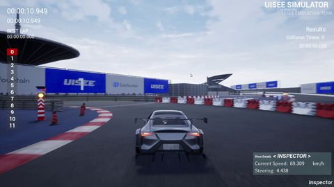
The task of the second round is to build a self-driving car in the UISEE simulator. The evaluation metric is the driving time of the car for completing the test track. The difficulties of this challenge is that only a driving simulator is provided by the organizer and the other tools such as data collection and control modules have to build by ourselves.
2.2 Driving Data Collection
First, we create a novel spatio-temporal driving dataset, called UISEE_SIM, in which the consecutive driving image sequences and corresponding driver behaviors (especially for the steer angles and driving speeds) are manually collected by a well-trained driver driving a racing car in the UISEE simulator.
The core contributions of this part are listed as follows:
- Different from the publicly driving dataset, our UISEE_SIM is a spatio-temporal dataset, i.e., all the images are consecutively, which enables that our driving model can extract motion cues from data and has a good performance on the task of speed prediction.
- Except to normal driving data, obstacle avoidance data also accounts for a large proportion, which helps the model acquires ability of recovering from mistakes and increases robustness of the driving system.
- The data collection tools can be found at
here and a better collection tool is contained in my
RoboCollectorproject.
UISEE_SIM
    ├── Stage-I
    │   ├── 20191118_label.txt
    │   ├── 20191120_label.txt
    │   ├── img
    │   └── label.txt
    ├── Stage-II
    │   ├── 20191121_label.txt
    │   ├── 20191122_label.txt
    │   ├── 20191204_label.txt
    │   ├── 20191205_label.txt
    │   ├── img
    │   └── label.txt
    ├── Stage-III
    │   ├── 20191206.csv
    │   ├── 20191208.csv
    │   ├── 20191209.csv
    │   ├── 20191210.csv
    │   ├── img
    │   └── label.csv
    └── test
        ├── img
        └── label.txt
2.3 Models
2.3.1 Modified PilotNet
The model we used here is the same as the one in the first round, except for the output module. Due to the difficulty of the speed prediction, we only predict steering angle control commands of the car and the speed control is implemented by a well-designed speed controller.
- The model code can be found at here
2.4 Training


- Normalize labels to [-1,1]
- Collecting more data at failed place
2.5 Control
$$
control.expected_speed = min(40, max(10, 25 + (1-abs(steer/2.0))*10.0))
        control.steering_angle = steer # angle
$$
2.6 Evaluation


2.7 Leaderboard
