1. Introduction
The simplest form of Imitation Learning is Behavior Cloning (BC), which focuses on learning the expert’s policy using supervised learning. Behavioral cloning is a method by which human sub-cognitive skills can be captured and reproduced in a computer program.
- As the human subject performs the skill, his or her actions are recorded along with the situation that gave rise to the action.
- A log of these records is used as input to a learning program.
- The learning program outputs a set of rules that reproduce the skilled behavior.
This method can be used to construct automatic control systems for complex tasks for which classical control theory is inadequate. It can also be used for training.
Synonyms:
- Apprenticeship learning;
- Behavioral cloning;
- Learning by demonstration;
- Learning by imitation;
- Learning control rules
In this project, we use deep convolutional neural networks to clone the driver’s behavior. The trained driving model outputs the steering angles to drive the car autonomously.
2. Related Work
2.1 ALVINN, an autonomous land vehicle in a neural network.
Dean A. Pomerleau. Technical report, Carnegie Mellon University, 1989. In many ways, DAVE-2 was inspired by the pioneering work of Pomerleau [1] who in 1989 built the Autonomous Land Vehicle in a Neural Network (ALVINN) system. It demonstrated that an end-to- end trained neural network can indeed steer a car on public roads. ALVINN used a fully-connected network which is tiny by today’s standard. Currently ALVINN takes images from a camera and a laser range finder as input and produces as output the direction the vehicle should travel in order to follow the road. Training has been conducted using simulated road images.

The input layer is divided into three sets of units: two “retinas” and a single intensity feedback unit. The two retinas correspond to the two forms of sensory input available on the NAVLAB vehicle; video and range information.
- The first retina, consisting of 30x32 units, receives video camera input from a road scene. The activation level of each unit in this retina is proportional to the intensity in the blue color band of the corresponding patch of the image. The blue band of the color image is used because it provides the highest contrast between the road and the non-road.
- The second retina, consisting of 8x32 units, receives input from a laser range finder. The activation level of each unit in this retina is proportional to the proximity of the corresponding area in the image.
- The road intensity feedback unit indicates whether the road is lighter or darker than the non-road in the previous image. Each of these 1217 input units is fully connected to the hidden layer of 29 units, which is in tum fully connected to the output layer. (Using this extra information concerning the relative brightness of the road and the non-road, the network is better able to determine the correct direction for the vehicle to travel.)
The output layer consists of 46 units, divided into two groups.
- The first set of 45 unitsis a linear representation of the tum curvature along which the vehicle should travel in order to head towards the road center.
- The middle unit represents the “travel straight ahead” condition while units to the left and right of the center represent successively sharper left and right turns.
- The final output unit is a road intensity feedback unit which indicates whether the road is lighter or darker than the non-road in the current image. During testing, the activation of the output road intensity feedback unit is recirculated to the input layer in the style of Jordan [Jordan, 1988] to aid the network’s processing by providing rudimentary infonnation concerning the relative intensities of the road and the non-road in the previous image.
The network is trained with a desired output vector of all zeros except for a “hill” of activation centered on the unit representing the correct turn curvature, which is the curvature which would bring the vehicle to the road center 7 meters ahead of its current position. More specifically, the desired activation levels for the nine units centered around the correct turn curvature unit are:
0.10, 0.32, 0.61, 0.89, 1.00, 0.89, 0.61, 0.32 0.10
During testing, the turn curvature dictated by the network is taken to be the curvature represented by the output unit with the highest activation level.
Training on actual road images is logistically difficult, because in order to develop a general representation, the network must be presented with a large number of training exemplaIS depicting roads under a wide variety of conditions. Collection of such a data set would be difficult, and changes in parameters such as camera orientation would require collecting an entirely new set of road images.
- To avoid these difficulties we have developed a simulated road generator which creates road images to be used as training exemplars for the network. Figure 2 depicts the video images of one real and one artificial road. Although not shown in Figure 2, the road generator also creates corresponding simulated range finder images. At the relatively low resolution being used it is difficult to distinguish between real and simulated roads.
- There are difficulties involved with training “on-the-fly” with real images.
- The range data contains information concerning the position of obstacles in the scene, but nothing explicit about the location of the road. do contribute to choosing the correct travel direction.
we would eventually like to integrate a map into the system to enable global point-to-point path planning.
2.2 End to End Learning for Self-Driving Cars
Bojarski, M.. 2016

Compared to explicit decomposition of the problem, such as lane marking detection, path planning, and control, our end-to-end system optimizes all processing steps simultaneously. We argue that this will eventually lead to better performance and smaller systems.
- Better performance will result because the internal components self-optimize to maximize overall system performance, instead of optimizing human-selected intermediate criteria, e. g., lane detection. Such criteria understandably are selected for ease of human interpretation which doesn’t automatically guarantee maximum system performance.
- Smaller networks are possible because the system learns to solve the problem with the minimal number of processing steps.
The groundwork for this project was done over 10 years ago in a Defense Advanced Research Projects Agency (DARPA) seedling project known as DARPA Autonomous Vehicle (DAVE) [2] in which a sub-scale radio control (RC) car drove through a junk-filled alley way. DAVE’s mean distance between crashes was about 20 meters in complex environments.
The primary motivation for this work is to avoid the need to recognize specific human-designated features, such as lane markings, guard rails, or other cars, and to avoid having to create a collection of “if, then, else” rules, based on observation of these features.

- Training data contains single images sampled from the video, paired with the corresponding steering command (1/r).
- Training with data from only the human driver is not sufficient. The network must learn how to recover from mistakes. Otherwise the car will slowly drift off the road.
- The training data is therefore augmented with additional images that show the car in different shifts from the center of the lane and rotations from the direction of the road.
- Images for two specific off-center shifts can be obtained from the left and the right camera. Additional shifts between the cameras and all rotations are simulated by viewpoint transformation of the image from the nearest camera. Precise viewpoint transformation requires 3D scene knowledge which we don’t have. We therefore approximate the transformation by assuming all points below the horizon are on flat ground and all points above the horizon are infinitely far away. This works fine for flat terrain but it introduces distortions for objects that stick above the ground, such as cars, poles, trees, and buildings. Fortunately these distortions don’t pose a big problem for network training. The steering label for transformed images is adjusted to one that would steer the vehicle back to the desired location and orientation in two seconds.
- In order to make our system independent of the car geometry, we represent the steering command as 1/r where r is the turning radius in meters. We use 1/r instead of r to prevent a singularity when driving straight (the turning radius for driving straight is infinity). 1/r smoothly transitions through zero from left turns (negative values) to right turns (positive values).
The network consists of 9 layers, including a normalization layer, 5 convolutional layers and 3 fully connected layers.

- The input image is split into YUV planes and passed to the network.
- The first layer of the network performs image normalization. The normalizer is hard-coded and is not adjusted in the learning process. Performing normalization in the network allows the normalization scheme to be altered with the network architecture and to be accelerated via GPU processing.
- We use strided convolutions in the first three convolutional layers with a 2×2 stride and a 5×5 kernel and a non-strided convolution (1 stride) with a 3×3 kernel size in the last two convolutional layers.
Training data was collected by driving on a wide variety of roads and in a diverse set of lighting and weather conditions.
- Most road data was collected in central New Jersey, although highway data was also collected from Illinois, Michigan, Pennsylvania, and New York.
- Other road types include: two-lane roads (with and without lane markings), residential roads with parked cars, tunnels, and unpaved roads.
- Data was collected in clear, cloudy, foggy, snowy, and rainy weather, both day and night. In some instances, the sun was low in the sky, resulting in glare reflecting from the road surface and scattering from the windshield.
- Our collected data is labeled with road type, weather condition, and the driver’s activity (staying in a lane, switching lanes, turning, and so forth).
We augment the data by adding artificial shifts and rotations to teach the network how to recover from a poor position or orientation. The magnitude of these perturbations is chosen randomly from a normal distribution.
- The distribution has zero mean, and the standard deviation is twice the standard deviation that we measured with human drivers.
- Artificially augmenting the data does add undesirable artifacts as the magnitude increases (see Section 2).
We estimate what percentage of the time the network could drive the car (autonomy). The metric is determined by counting simulated human interventions (see Section 6). These interventions occur when the simulated vehicle departs from the center line by more than one meter. We assume that in real life an actual intervention would require a total of six seconds: this is the time required for a human to retake control of the vehicle, re-center it, and then restart the self-steering mode. $$ autonomy = (1-\frac{(number\ of\ interventions)\cdot 6\ seconds}{elapsed\ time\ [seconds]})\cdot 100 $$
3. Dataset
3.1 Data Collection
I use image data and steering angles which are collected in the Udacity simulator to train a neural network and then use this model to drive the car autonomously around the track in simulator.
- At first, I gathered 1438 images from a full lap around track. But I can not always keep the car driving at the center line of the road. This is not a good dataset and some previous experience have shown that this kind of data will make the car pull too hard while testing. So I discard it.
- Then I collected a new dataset which contains 2791(x3) images by driving the car travel the full track two times.
- The total numbers of images are about 8000 by counting two side images
- The couple of problem areas on each track were addressed by training the vehicle recovering from the sides of the road.
tips:
- use left and right images and their corresponding steering angle is the original steering angle adding (left) or subtracting (right) a correction angle
- collecting more data at the easily failed place such as the turn track.
- Collecting the revise driving data
3.2 Data Preprocessing
Images were preprocessed before feeding to the neural network.
Color Space
There are three types of color space for image representation. I tried different color spaces and found that the model generalized best using images in the BGR color space.

- Conversion to BGR color space solved both of these issues and required less training files overall.
- Training with the YUV color space gave erratic steering corrections resulting in too much side-to-side movement of the car. (test)
- In the RGB color space some areas of track required many more training images to navigate correctly, particularly the areas with dirt patches on the side of the road. (test)
Notes:
- Please keep in mind that the colorspace of training images loaded by cv2 is BGR. However, when the trained network predicts the steering angles at the testing stage,
drive.pyloads images with RGB colorspace.
Image Cropping
I crop the unnecessary portions of the image (background of sky, trees, mountains, hood of car) taking 50 pixels off the top of the image and 20 pixels off the bottom.

image = cv2.cvtColor(image, cv2.COLOR_BGR2RGB)
model = Sequential()
model.add(Cropping2D(cropping=((50, 20),(0,0)), input_shape=(160,320,3)))

# output the intermediate layer!
## can be used to show learned features for any layer
layer_output = backend.function([model.layers[0].input], [model.layers[0].output])

# note that the shape of the image suited for the network!
cropped_image = layer_output([image[None,...]])[0][0]

# convert to uint8 for visualization
cropped_image = np.uint8(cropped_image)
Image Resizing
The cropped image is then resized to (128, 128) for input into the model. I found that resizing the images decreased training time with no effect on accuracy.
3.3 Data Augmentation
There are four kinds of methods for data augmentation. Images could be augmented by
- flipping horizontally,
- blurring,
- changing the overall brightness,
- or applying shadows to a portion of the image.
When reading original data from CSV file, flipped_flag, shadow_flag, bright_flag, blur_flag will be assigned to each image. The image processing will be done when generating practical data sets.
Randomly changing the images to augment the data set was not only was not necessary but when using the RGB color space I saw a loss of accuracy.
Flipping horizontally
By adding a flipped image for every original image the data set size was effectively doubled. When reading original data from the CSV file, the path of the flipped image is the same as the original image. However, a flipped flag (equals to 1) will be assigned to the flipped image and the flag of the original image is 0. Finally, the corresponding flipping operation will be done for each image according to this flag. Meanwhile, we set the negative value of the label which corresponds to the original image as the label of the flipped image.
Changing brightness

Bluring

kernel_size = (np.random.randint(1,5)*2) +1
blur = cv2.GaussianBlur(rgb, (kernel_size,kernel_size), 0)
Random shadow

See the functions random_blur(), random_brightness(), and random_shadow() in the file data.py for augmentation code.
Balance Data Distribution
One improvement that was found to be particularly effective was to fix the poor distribution of the data. A disproportionate number of steering angles in the data set are at or near zero. To correct this:
- steering angles are separated into 25 bins.
- Bins with a count less than the mean are augmented
- while bins with counts greater than the mean are randomly pruned to bring their counts down.
- Those operations equalize the distribution of steering angles across all bins.


4. Model
4.1 Fully Connected Model
I tried a fully connected neural network with one hidden layer (100 units).
At first, the normalization layer is not used in this model. The mae loss of the network is decreased to 2 after 10 epochs of training (the mse loss is about 40). However, the predicted steering angles are very large (30~40) resulting in that the car drives out of the track.
- Then I tried to increase training epochs. The network is overfitting after two epochs. The predicted steering angles are always 0 while testing.
- Then I trained the network again without any parameter adjustment. The training process is normal and the final loss seems reasonable to drive the car autonomously. However, the testing result is bad.
After above attempts, A normalization layer was added to the network. The mse loss decreased to 8.8145 and the mae loss decreased to 1.9536. It is worth noting that the mae loss almost no longer reduced after 10 training epochs. Finally, the car can drive at the straight track but the steering angle is still too large at the turn of the track.
- The parameter file is saved as
fcnet-normalize.h5 - Then i trained again with the same setup, The result seems very similar to the last traing. However, the initial predicted steering angle is too large to drive the car out of the track.
- May be I should collect more images to improve the robustness of the network.
- Based on the above setup, the hidden layer units are increased to 1000 from 100. But the network converge more slowly and the final results is not good at all. The predicted steering angles is about 7.
4.2 Nvidia PilotNet
The model and training process are listed below. The final trained model is very well. All the saved model (even the model saved after 1 epoch) can keep the car drving along the center line of the track for the full lap without any fails. The desired velocity of the car can be set arbitrary from 0 to 30.
Reading data from csv file...
Reading is done.
EPOCHS: 20
Training Set Size: 6698
Valization Set Size: 1675
Batch Size: 256
/home/ubuntu16/Behavioral_Cloning/data.py:102: RuntimeWarning: divide by zero encountered in true_divide
  copy_times = np.float32((desired_per_bin-hist)/hist)
Training set size now: 6122
Using TensorFlow backend.
_________________________________________________________________
Layer (type)                 Output Shape              Param #
=================================================================
cropping2d_1 (Cropping2D)    (None, 90, 320, 3)        0
_________________________________________________________________
lambda_1 (Lambda)            (None, 90, 320, 3)        0
_________________________________________________________________
conv2d_1 (Conv2D)            (None, 43, 158, 24)       1824
_________________________________________________________________
conv2d_2 (Conv2D)            (None, 20, 77, 36)        21636
_________________________________________________________________
conv2d_3 (Conv2D)            (None, 8, 37, 48)         43248
_________________________________________________________________
conv2d_4 (Conv2D)            (None, 6, 35, 64)         27712
_________________________________________________________________
conv2d_5 (Conv2D)            (None, 4, 33, 64)         36928
_________________________________________________________________
flatten_1 (Flatten)          (None, 8448)              0
_________________________________________________________________
dense_1 (Dense)              (None, 1164)              9834636
_________________________________________________________________
dense_2 (Dense)              (None, 100)               116500
_________________________________________________________________
dense_3 (Dense)              (None, 50)                5050
_________________________________________________________________
dense_4 (Dense)              (None, 10)                510
_________________________________________________________________
dense_5 (Dense)              (None, 1)                 11
=================================================================
Total params: 10,088,055
Trainable params: 10,088,055
Non-trainable params: 0
_________________________________________________________________
Training with 24 steps, 7 validation steps.
Epoch 1/20
24/24 [==============================] - 11s 438ms/step - loss: 0.2917 - mean_absolute_error: 0.4121 - val_loss: 0.0490 - val_mean_absolute_error: 0.1765
Epoch 2/20
24/24 [==============================] - 9s 395ms/step - loss: 0.0581 - mean_absolute_error: 0.1890 - val_loss: 0.0403 - val_mean_absolute_error: 0.1485
Epoch 20/20
24/24 [==============================] - 10s 400ms/step - loss: 0.0043 - mean_absolute_error: 0.0484 - val_loss: 0.0203 - val_mean_absolute_error: 0.1128
4.3 Modified NVIDIA Network
Overall, The modified nvidia network is very similar to the original one.
- In this version, all the strides of filters are set to be 1. The corresponding max pooling operation is added after the first three convolution layers to ensure the output is consistent with the original network.
- Dropout layers were used in between the fully connected layers to reduce overfitting.
- The final performance of the trained network is almost the same as the original one.
The final network is as follows:
| Layer | Output Shape | Param # |
|---|---|---|
| Normalization (Lambda) | (128, 128, 3) | 0 |
| 1st Convolutional/ReLU | (124, 124, 24) | 1824 |
| Max Pooling | (62, 62, 24) | 0 |
| 2nd Convolutional/ReLU | (58, 58, 36) | 21636 |
| Max Pooling | (29, 29, 36) | 0 |
| 3rd Convolutional/ReLU | (25, 25, 48) | 43248 |
| Max Pooling | (12, 12, 48) | 0 |
| 4th Convolutional/ReLU | (10, 10, 64) | 27712 |
| 5th Convolutional/ReLU | (8, 8, 64) | 36928 |
| Flatten | (4096) | 0 |
| Dropout | (4096) | 0 |
| 1st Fully Connected | (1164) | 4768908 |
| Dropout | (1164) | 0 |
| 2nd Fully Connected | (100) | 116500 |
| 3rd Fully Connected | (50) | 5050 |
| 4th Fully Connected | (10) | 510 |
| 5th Fully Connected | (1) | 11 |
Training:
25/25 [==============================] - 13s 503ms/step - loss: 0.2863 - mean_absolute_error: 0.4376 - val_loss: 0.1224 - val_mean_absolute_error: 0.2843
Epoch 2/20
25/25 [==============================] - 10s 417ms/step - loss: 0.0728 - mean_absolute_error: 0.2170 - val_loss: 0.0419 - val_mean_absolute_error: 0.1532
Epoch 20/20
25/25 [==============================] - 10s 415ms/step - loss: 0.0152 - mean_absolute_error: 0.0967 - val_loss: 0.0250 - val_mean_absolute_error: 0.1219
To train a CNN to do lane following we only select data where the driver was staying in a lane and discard the rest.
- We then sample that video at 10 FPS. A higher sampling rate would result in including images that are highly similar and thus not provide much useful information.
- To remove a bias towards driving straight the training data includes a higher proportion of frames that represent road curves.
5. Experiments
5.1 Experimental results of Fully Connected Network

5.2 Experimental results of PilotNet

5.3 Experimental results of our Modified PilotNet

tips:
- The trained network can drive the car across the full tack with 9 mph.
- Two laps of track images are used. The distribution of the data was fixed duiring training. The data set did not flipped.
- You must make the car driving along the center of the track. Otherwise, the car will drive out of the track will testing.
- finall loss is 0.02
6. Related Projects
6.1 Open Source Self-Driving Car Project
This project is maintained by Udacity and the aim of this project is to create a complete autonomous self-driving car using deep learning and using ROS as middleware for communication.
Sensors and components used in the Udacity self-driving car:
- 2016 Lincoln MKZ :
- Two Velodyne VLP-16 LiDARs
- Delphi radar
- Point Grey Blackfly cameras
- Xsens IMU
- Engine control unit ( ECU )
dbw_mkz_ros package:
- This project uses the dbw_mkz_ros package to communicate from ROS to the Lincoln MKZ. In the previous section, we set up and worked with the dbw_mkz_ros package.
- Here is the link to obtain a dataset for training the steering model: https://github.com/udacity/self-driving-car/tree/master/datasets . You will get a ROS launch file from this link to play with these bag files too.
- Here is the link to get an already trained model that can only be used for research purposes: https://github.com/udacity/self-driving-car/tree/master/steering-models . There is a ROS node for sending steering commands from the trained model to the Lincoln MKZ.
- Here, dbw_mkz_ros packages act as an intermediate layer between the trained model commands and the actual car.
- reference to implement the driving model using deep learning and the entire explanation for it are at https://github.com/thomasantony/sdc-live-trainer .
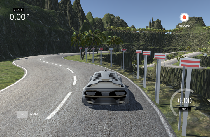
This simulator was built for Udacity’s Self-Driving Car Nanodegree, to teach students how to train cars how to navigate road courses using deep learning.
See more project details here. All the assets in this repository require Unity. Please follow the instructions below for the full setup.
Term 1
- Instructions: Download the zip file, extract it and run the executable file.
- Version 2, 2/07/17 Linux Mac Windows
- Version 1, 12/09/16 Linux Mac Windows 32 Windows 64
Term 2
- Please see the Releases page for the latest version of the Term 2 simulator (v1.45, 6/14/17).
- Source code can be obtained therein or also on the term2_collection branch.
Term 3
- Please see the Releases page for the latest version of the Term 3 simulator (v1.2, 7/11/17).
- Source code can be obtained therein or also on the term3_collection branch.
System Integration / Capstone
- Please see the CarND-Capstone Releases page for the latest version of the Capstone simulator (v1.3, 12/7/17). Source code can be obtained therein.
Unity Simulator User Instructions (for advanced development)
- Clone the repository to your local directory, please make sure to use Git LFS to properly pull over large texture and model assets.
- Install the free game making engine Unity, if you dont already have it. Unity is necessary to load all the assets.
- Load Unity, Pick load exiting project and choice the
self-driving-car-simfolder. - Load up scenes by going to Project tab in the bottom left, and navigating to the folder Assets/1_SelfDrivingCar/Scenes. To load up one of the scenes, for example the Lake Track, double click the file LakeTrackTraining.unity. Once the scene is loaded up you can fly around it in the scene viewing window by holding mouse right click to turn, and mouse scroll to zoom.
- Play a scene. Jump into game mode anytime by simply clicking the top play button arrow right above the viewing window.
- View Scripts. Scripts are what make all the different mechanics of the simulator work and they are located in two different directories, the first is Assets/1_SelfDrivingCar/Scripts which mostly relate to the UI and socket connections. The second directory for scripts is Assets/Standard Assets/Vehicle/Car/Scripts and they control all the different interactions with the car.
- Building a new track. You can easily build a new track by using the prebuilt road prefabs located in Assets/RoadKit/Prefabs click and drag the road prefab pieces onto the editor, you can snap road pieces together easily by using vertex snapping by holding down “v” and dragging a road piece close to another piece.
Related Resources: